My Renderer with Fog

Introduction

Imagine exploring the eerie remains of a sunken ship in a deep-sea game, your flashlight revealing lost treasures in the shadows. Picture a horror game where a fog shrouds a mysterious town, and you cautiously navigate the dimly lit streets. In these gaming scenarios, light interacts with scattering media, creating atmospheric effects that add depth and realism. This project implements a renderer based on ray tracing and statistical simulation of cloud media.

More theoretical and engineering detail in

My paper: https://github.com/58191554/FogRenderer/blob/main/Fog_Renderer.pdf

Github original code: https://github.com/58191554/FogRenderer/tree/main

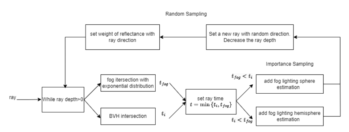
Based on the ray tracer, the fog renderer is implemented by two part, the fog particle intersection and fog scattering.

Particle Intersection

First, we assume the fog particle is uniformly distributed in the atmosphere. The ray will hit fog particles before intersecting with the object. To define when the ray hit the particle, exponential distribution is used to describe the probability of a time interval between two event (ray hit particle). Taking the inverse of exponential distribution CDF, we can sample the fog with the same sample rate of no fog, and reach a fog-blur effect.

According to the definition of the Poisson process, the time interval between the $k^{th}$ random event and the $k+1^{th}$ random event follows an exponential distribution [Eric P. Lafortune and Yves D. Willems]. And the probability of zero random events occurring in a time period of length $t$ is equal to

P(t|\text{hit}=0)=\frac{e^{-\lambda t}(\lambda t)^0}{0!} = e^{-\lambda t}\\P(t|\text{hit}>0) = 1-e^{-\lambda t}

CDF of exponential distribution:

\frac{dL}{dt} = -\sigma_t(t) L dt \\L = L_0 e^{-\int_{t_0}^{t_{end}} \sigma_t(x) \, dx} = L_0 e^{-\sigma_t t_{end}}

$dL$ is the light intensity derivative, and $dt$ is the time derivative along the ray. $\sigma_t = \sigma_a + \sigma_s$ is the sum of the absorption and out-scattering coefficients. The first equation describes the decay of the intensity $L$ when the ray goes through place $\vec{o} + \vec{d}t$ the absorbing and out-scattering media. Solving the equation, we get the integrated formula that can tell us how much light after decay we observe by the intersection $t_{end}$

Fog Scattering

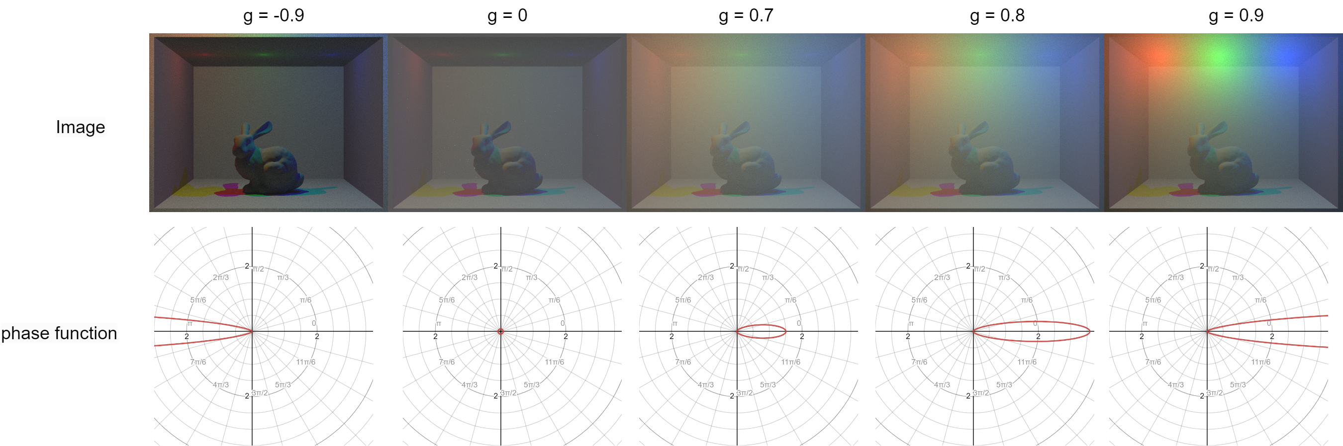
After the fog particle intersection, we need to implement fog particle reflect the light. By Monte Carlo sampling, we can have different probabilities among directions. According to the Henyey-Greenstein phase function,

P_{HG}(\theta) = \frac{1}{4\pi} \frac{1 - g^2}{(1 + g^2 - 2g \cos \theta)^{3/2}}

Setting the different values of g, we can probability distribution with $θ$ , the ray direction is from the negative side of the polar axis. When $g = 0$ , the BSDF is diffuse-like; when $g$ is negative, the ray transmits forward; and when g is positive, the ray reflects backward.

With different g, we can render different effects of fog. From the showcase below, we can see the fog particle below the light is observed, while the fog particle far from the light is less visible since there is little reflection on the camera.

In the images above, the first image is the function shape in polar space, and the radius represents the probability. The second image is 3 point lights of red, green, and blue. The third image is an area of light, and the fourth image is a spotlight

Implementation Details

This project implements all the algorithms in C++. It is based on the third assignment starter code provided by the University of California, Berkeley’s CS184 course.The first step involves reading the DAE (Digital Asset Exchange) file, which contains the 3D scene data.After reading the object from the file, the next step is to perform BVH. Once the BVH segmentation is done, rays are cast into the scene. The number of rays emitted is determined by the sample rate and sample light size settings. If thin lens parameters are used, lens sampling is performed during ray generation to achieve Depth of Field (DOF) effect.During ray casting, collision detection with scene objects is performed, and the material parameters and BSDF of the colliding surface are accessed by the ray. The rays are then sampled for reflection or refraction based on the BSDF. When there is a glass object, we apply Schlick’s Approximation[ 12 ]. If importance sampling is enabled, the algorithm iterates through all light sources and samples rays accordingly

Performance and Image Result

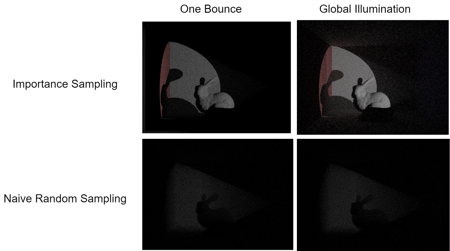
One-Bounce & Global Illumination

We have achieved global illumination in our rendering, allowing spotlights to illuminate walls outside their direct range, and the shadowed areas now have increased brightness (they are not completely black anymore). By employing light direction importance sampling, we have significantly improved the quality of the rendered images. As shown in the images, without importance sampling, the rendering appears completely dark with low sample counts and exhibits significant noise at high sample counts

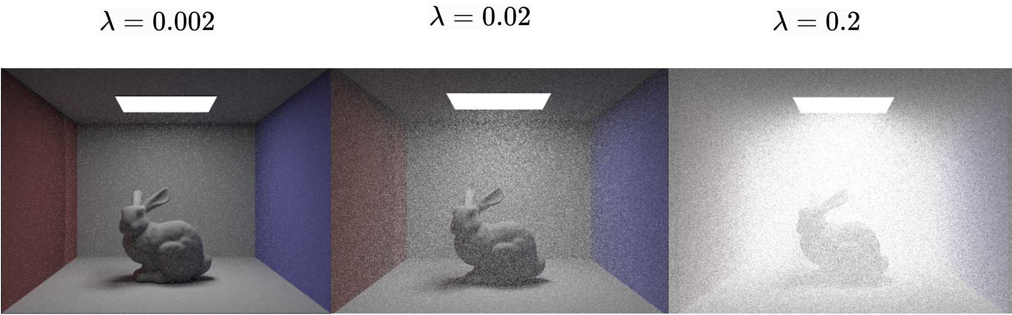
Different Density Parameter & Phase Parameter

After continuously adjusting the value of lambda λ, it was found that lambda between 0.02 and 0.2 produces a fog effect that closely resembles reality.

As shown in the figure, different values of the parameter "g" ranging from -1 to 1 result in varying effects of fog on light in different directions. The image displays distinct results for selected values of "g." For values of "g" less than 0, the differences are not significant, as the scene appears elatively dark overall. In the range of "g" values greater than 0 and less than 0.6, the differences are not substantial, and the scene appears to have a milky white appearance. However, when "g" is set to 0.9, a phenomenon of a "halo" around the light source becomes evident, where the area surrounding the light source appears brighter than the rest of the scene.

Phase function changing

RGB top spot light scene changes with phase function

Eight Bounce

Global Bounce

References

[1] J. Arvo and D. Kirk. Fast ray tracing by ray classification. ACM Siggraph Computer Graphics,

21(4):55–64, 1987.

[2] B. Foundation. Blender - a 3d modeling and rendering software. https://www.blender.

org/.

[3] L. G. Henyey and J. L. Greenstein. Diffuse radiation in the galaxy. Astrophysical Journal,

93:70–83, 1941.

[4] W. Jarosz. Efficient Monte Carlo methods for light transport in scattering media. PhD thesis,

University of California, San Diego, 2008.

[5] W. Jarosz, H. W. Jensen, H. Moreton, and J. Stam. A comprehensive theory of volumetric

radiance estimation using photon points and beams. ACM Transactions on Graphics (TOG),

30(1):1–19, 2011.

[6] H. W. Jensen and J. Buhler. A practical model for subsurface light transport. In Proceedings of

the 28th Annual Conference on Computer Graphics and Interactive Techniques, 2001.

[7] H. W. Jensen, P. H. Christensen, and E. Chan. A practical guide to global illumination using ray

tracing and photon mapping. SIGGRAPH Course Notes, 2001.

[8] J. T. Kajiya. The rendering equation. In Proceedings of the 13th Annual Conference on

Computer Graphics and Interactive Techniques, 1986.

[9] E. P. Lafortune and Y. D. Willems. Rendering participating media with bidirectional path tracing.

In S. N. Spencer, editor, Rendering Techniques ’96: Proceedings of the Eurographics Workshop,

page 7, Porto, Portugal, June 1996. Springer Vienna.

[10] F. E. Nicodemus. Directional reflectance and emissivity of an opaque surface. Applied Optics,

4(7):767–775, 1965.

[11] M. Pharr and G. Humphreys. Physically Based Rendering: From Theory to Implementation.

Morgan Kaufmann, 2010.

[12] C. Schlick. An inexpensive brdf model for physically-based rendering. Computer graphics

forum, 13(3), 1994.

[13] C. University. Cornell box. Online, 1984.

[14] S. University. The stanford 3d scanning repository. http://graphics.stanford.edu/

data/3Dscanrep/.

[15] J. Zhang. On sampling of scattering phase functions. Astronomy and Computing, 29:100329,

2019.