A notebook, taken apart · Generative modeling
DDPM, train your MNIST generator
Train a conditional diffusion model on MNIST—and inspect what “learning to denoise” actually means.
I thought diffusion sounded intuitive: add noise to an image, learn to remove it, and eventually generate images from randomness. Then I tried to implement a model that takes a digit label and produces a handwritten digit. The slogan left almost every engineering question unanswered. What is the training target? Where do we get it? Does each update run through all the denoising steps? And why would predicting random noise teach a model anything about handwriting?
This post follows my diffusion_tut.ipynb and its utils.py, in their original order: data, noise schedule, embeddings, residual blocks, U-Net, loss, training, checkpoint, and sampling. The recorded notebook preserves the completed Colab T4 run, including its training logs and generated images. The separate self-contained training edition places the helpers directly in the notebook so you can train your own model without my Drive folder. You should be comfortable with tensors, convolutions, and backpropagation; the diffusion-specific details are developed below.
1. Run your own copy
- Click Open in Colab to open
train_in_colab.ipynb, then File → Save a copy in Drive. Alternatively, download the.ipynband upload it through Colab's notebook picker. - Select a GPU under Runtime → Change runtime type. Run the setup cell and check the printed device and library versions. CPU is sufficient for the small shape checks; use a GPU for the full training run. Colab's resources and runtime limits vary, so a 300-epoch run may span sessions. See the Colab FAQ.
- Run the cells from top to bottom. The notebook contains the helper code; there is no
sys.pathedit, required Drive mount, or separate Python file to upload. MNIST downloads when the data cell runs. - For a first execution check, change
cfg.epochsto1before the training cell. That checks the workflow; it is not a claim that one epoch produces a good generator. KeepT=300and the architecture unchanged. Use the originalepochs=300configuration for the longer baseline experiment. - The training cell saves a checkpoint after each epoch. Its default path is local to the runtime. Use the optional Drive cell before training, or download the checkpoint before disconnecting. To continue later, run setup and the model definitions, set the same checkpoint path, and enable the resume flag in the training cell.
The self-contained training edition prints the package versions actually used in your session. Seeds make comparisons easier, but do not guarantee identical results across hardware and library versions. GPU memory use also depends on your runtime; if necessary reduce the batch size, and keep that change in your experiment notes.
2. Configuration and MNIST
The configuration currently written in the source notebook is small in image size, but not a tiny number of optimization steps:
| Setting | Notebook value | Meaning |
|---|---|---|
| Image / classes | 1 × 28 × 28, 10 |
Grayscale images, labels 0 through 9 |
| Batch / loader workers | 128, 2 |
Images per update and data-loading workers |
Diffusion steps T |
300 |
Noise levels indexed from 0 through 299 |
| Learning rate / epochs | 1e-4, 300 |
AdamW step size and full dataset passes |
| Base channels | 64 |
First encoder block width |
| Time embedding dimension | 128 |
Width of the combined condition vector |
| Checkpoint | ./mnist_cond_ddpm.pt |
Default runtime-local output |
An epoch and a diffusion timestep are different things. MNIST has 60,000 training images. With batches of 128 and no dropped final batch, there are 469 optimizer updates per epoch; the final batch contains 96 images. Three hundred epochs therefore mean 140,700 training updates. The coincidence that both epochs and T equal 300 has no algorithmic significance.
transform = transforms.Compose([
    transforms.ToTensor(),
    transforms.Lambda(lambda x: x * 2.0 - 1.0),
])
train_dataset = datasets.MNIST(
    root=cfg.data_dir, train=True, download=True, transform=transform,
)
train_loader = DataLoader(
    train_dataset, batch_size=cfg.batch_size, shuffle=True,
    num_workers=cfg.num_workers, pin_memory=(device == "cuda"),
)
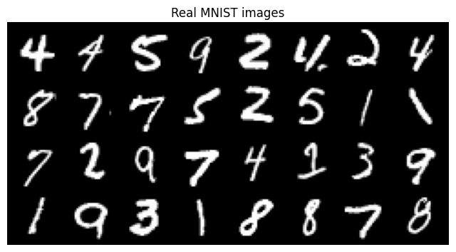
ToTensor() gives floating-point pixels in [0, 1]; the next transform maps black to -1 and white to 1. This establishes a convenient image scale relative to unit Gaussian noise. It does not make MNIST zero-mean or unit-variance. Most MNIST pixels are background, so symmetric endpoints alone do not center the data distribution.
A batch x0 has shape [B, 1, 28, 28]; y has shape [B] and integer dtype. Labels remain integers for the embedding lookup. show_images reverses the pixel scaling with (images + 1) / 2, clamps only for display, and assembles a grid. The original helper accepts a labels argument but does not draw label captions.
3. Build the forward noise process
3.1 Start with one transition
For the derivation only, let k count physical noising steps starting at 1, and let x0 be the clean image. One step is:
The image and noise are multiplied by square roots because their variances scale with the square of those coefficients. Conditional on the previous image, the added noise has variance βk. If the previous random image had variance 1 and were independent of the new noise, the resulting variance would also be 1. That is a conditional statement about the input distribution, not a property guaranteed by the MNIST transform.
Expanding two steps explains the cumulative product:
The two independent Gaussian terms combine into a Gaussian with variance α2β1 + β2 = 1 − α1α2. Repeating the same reasoning gives:
The ε here represents the combined noise at that level, not just the last incremental noise draw. The equality is a statement about the conditional distribution; drawing a fresh ε reproduces that marginal without replaying the same trajectory. This is the closed-form forward marginal in DDPM, Equation 4.
This is the computational payoff: after precomputing the schedule in O(T), creating a training image at any selected level takes one tensor expression. It is constant work in the number of diffusion steps, while still scaling with the number of pixels. Training does not have to simulate hundreds of forward transitions per image.
3.2 Translate the math into zero-based code
The notebook uses array indices t=0,...,T-1. Thus schedule["alpha_bars"][t] is the product through array element t inclusive; code index t corresponds to physical step k=t+1. The variable named x_t is already slightly noisy when t=0. It is not the clean x0. At sampling index 0, the reverse step returns the final image.
betas = torch.linspace(1e-4, 0.02, T, device=device)
alphas = 1.0 - betas
alpha_bars = torch.cumprod(alphas, dim=0)
sqrt_alpha_bars = torch.sqrt(alpha_bars)
sqrt_one_minus_alpha_bars = torch.sqrt(1.0 - alpha_bars)
sqrt_recip_alphas = torch.sqrt(1.0 / alphas)
All six arrays have shape [T]. Beta increases linearly; alpha decreases linearly. Alpha-bar decreases multiplicatively. These are fixed tensors, not learned parameters. The schedule dictionary caches both the forward coefficients and the reciprocal-alpha factor used later by the sampler.
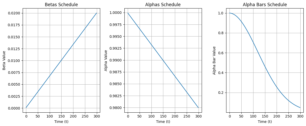
For this particular 300-step schedule, the last α-bar is approximately 0.04806, so its square root is approximately 0.2192. The noise coefficient is approximately 0.9757. There is still a scaled image component at the last training level. Starting generation from an exact standard Gaussian therefore introduces a terminal-distribution approximation. The tutorial retains the original schedule; it does not silently substitute a longer one.
3.3 Select a different noise level for each image
def extract(a, t, x_shape):
    values = a.gather(0, t)                 # [B]
    return values.reshape(t.shape[0], *([1] * (len(x_shape) - 1)))

noise = torch.randn_like(x0)               # [B, 1, 28, 28]
t = torch.randint(0, cfg.T, (x0.shape[0],), device=x0.device)
a = extract(schedule["sqrt_alpha_bars"], t, x0.shape)
b = extract(schedule["sqrt_one_minus_alpha_bars"], t, x0.shape)
x_t = a * x0 + b * noise
gather selects one schedule coefficient per sample. Reshaping [B] to [B, 1, 1, 1] makes broadcasting apply that coefficient to every pixel of its own image. Without that reshape, PyTorch aligns dimensions from the right; a batch dimension is not automatically treated as the first image axis. The schedule, timestep indices, and images must share a device.

4. Encode time and the requested digit
A noisy tensor alone does not reliably identify its noise level. The network also needs to distinguish “denoise this into a seven” from the same request for a zero. The notebook supplies both pieces of information through a vector of width 128.
4.1 Sinusoidal timestep embedding
For dim=128, there are 64 frequencies. The implementation uses raw integer timesteps, not timesteps divided by T:
half_dim = dim // 2
freqs = torch.exp(
    -math.log(10000) * torch.arange(
        half_dim, device=t.device, dtype=torch.float32
    ) / (half_dim - 1)
)
args = t.float()[:, None] * freqs[None, :]
emb = torch.cat([torch.sin(args), torch.cos(args)], dim=-1)
The frequencies run from 1 down to 0.0001. Multiplying [B, 1] by [1, 64] produces [B, 64]; concatenation gives [B, 128]. The first half is sine, and the second half is cosine. At t=0, the first 64 entries are zero and the last 64 are one. The original notebook checks [0, 1, 10, 100], the resulting shape [4, 128], and several numerical values. These checks catch a changed frequency scale or concatenation order. The helper also pads odd widths; use the baseline width of 128 here.
4.2 Add the label embedding
t_emb = self.time_mlp(sinusoidal_time_embedding(t, 128))
y_emb = self.label_emb(y)
emb = t_emb + y_emb
The time MLP is Linear(128, 512) → SiLU → Linear(512, 128). The label table is Embedding(10, 128): each digit selects one learned row. The sinusoidal encoding is fixed; the MLP and label table are optimized through the denoising loss. Addition preserves [B, 128]; concatenation would produce 256 features and require changing every subsequent projection.
This is direct class conditioning. There is no label dropout, unconditional branch, external digit classifier, or guidance scale in this implementation. Those would be additional mechanisms; classifier-free guidance, for example, combines conditional and unconditional predictions.
5. Trace every U-Net tensor
5.1 What one residual block does
h = self.conv1(x)                          # in_ch → out_ch, 3×3
emb_out = self.emb_proj(emb)[:, :, None, None]
h = self.act(h + emb_out)                  # broadcast over H and W
h = self.act(self.conv2(h))                # out_ch → out_ch, 3×3
return h + self.skip(x)
Both convolutions use padding 1, so they preserve spatial size. emb_proj maps 128 condition features to out_ch; the result becomes [B, out_ch, 1, 1]. Adding it is a learned channel-wise offset shared across spatial positions. The surrounding convolutions can respond differently to image content under different conditions.
If in_ch == out_ch, the residual skip is an identity. Otherwise, a learned 1×1 convolution changes its channel count. The addition requires matching dimensions. This local residual addition is distinct from the U-Net's later encoder-to-decoder concatenations.
The original checks explicitly exercise 1→64, 64→64, and 64→128 channels on four 28×28 inputs. Expected outputs are [4,64,28,28], [4,64,28,28], and [4,128,28,28]. This implementation has SiLU activations but no batch normalization, group normalization, attention, or dropout.
5.2 Follow the encoder and decoder
| Operation | Output shape | What is retained or combined |
|---|---|---|
| Noisy input | [B,1,28,28] |
The image at the sampled noise level |
down_block1 |
[B,64,28,28] |
Save this as h1 |
downsample1 |
[B,64,14,14] |
4×4 convolution, stride 2, padding 1 |
down_block2 |
[B,128,14,14] |
Save this as h2 |
downsample2 |
[B,128,7,7] |
Same spatial reduction |
mid_block |
[B,128,7,7] |
Process the coarsest features |
upsample1 |
[B,128,14,14] |
Nearest-neighbor resize ×2, then 3×3 convolution |
Concatenate with h2 |
[B,256,14,14] |
torch.cat(..., dim=1) |
up_block1 |
[B,64,14,14] |
Reduce 256 channels to 64 |
upsample2 |
[B,64,28,28] |
Resize ×2, then 3×3 convolution |
Concatenate with h1 |
[B,128,28,28] |
Recover features at the original resolution |
up_block2 |
[B,64,28,28] |
Combine coarse and fine information |
out_conv |
[B,1,28,28] |
Linear 1×1 projection to predicted noise |
The coarse features provide spatial context; the stored encoder features preserve detail at each resolution. Because 28→14→7→14→28 matches exactly, this architecture does not need cropping to join its skips. At the baseline widths, the model has 1,585,729 trainable parameters. The final convolution has no sigmoid or tanh: Gaussian noise is not restricted to [0,1] or [-1,1].
6. Understand the noise-prediction objective
6.1 Build one supervised training example
B = x0.shape[0]
t = torch.randint(0, cfg.T, (B,), device=x0.device)
noise = torch.randn_like(x0)
x_t = add_noise(x0, t, noise, schedule)
pred_noise = model(x_t, t, y)
loss = F.mse_loss(pred_noise, noise)
There is no missing ground truth: we draw noise ourselves and keep it. The clean image participates in constructing the input, but it is not directly supplied to the network. The target is the unscaled noise, not b * noise, x0, or the preceding noisy image.
Each example gets its own uniformly sampled t. A single batch can contain nearly clean images and heavily corrupted images together. A later visit to the same digit image usually draws a new timestep and a new noise tensor. There is one U-Net call per training batch, not 300 sequential denoising calls.
F.mse_loss averages squared errors over batch, channel, height, and width. A full batch therefore averages 100,352 scalar errors. In expectation over the images, times, and Gaussian draws, the objective is:
This follows the simplified noise-prediction objective discussed in DDPM, Section 3.4. The helper does not compute the complete variational bound or introduce explicit per-timestep loss weights.
6.2 Why “the noise is random” does not make this impossible
Before constructing x_t, the noise is independent of the training image. After constructing x_t, it is part of what the network observes. The task is to estimate which part of this observation can be explained by noise, given the noise level and the distribution of images with that label.
For squared error, the best possible predictor at a given input is the conditional mean:
This follows directly from minimizing expected squared error: the error separates into irreducible conditional variance and squared distance from the conditional mean. Several clean images and noise realizations can explain a similar noisy observation, so the model need not recover each exact random draw perfectly. Learning across many such examples teaches it which spatial patterns are plausible handwriting.
A useful diagnostic is the implied clean-image estimate:
Here and below, the coefficients use the notebook's zero-based array index convention. Replacing the prediction with the exact training noise reconstructs x0 up to floating-point error. Replacing it with an imperfect prediction shows why high noise levels are difficult: the error is multiplied by √((1−α-bar)/α-bar), about 4.45 at index 299. Small noise MSE can still correspond to a visibly imperfect clean estimate.
6.3 Interpret the initial loss correctly
The recorded T4 notebook shows 1.0472511053085327 before training and 1.0450210571289062 in its backward-pass check. A predictor that always outputs zero has expected MSE 1 against standard Gaussian noise. A randomly initialized network with modest outputs can therefore start near 1, but its output is not guaranteed to be zero and its loss is not guaranteed to equal 1.
These two numbers are sanity-check observations, not a learning curve: they use different random examples, and the backward-check loss is computed before its optimizer update. A shape match and a loss near 1 verify parts of the wiring, not denoising quality.
7. Train, save, and reload
The original backward check creates AdamW, computes one loss, clears gradients, backpropagates, and steps the optimizer:
optimizer = torch.optim.AdamW(model.parameters(), lr=cfg.lr)
loss = diffusion_loss(model, x0, y, schedule, cfg)
optimizer.zero_grad()
loss.backward()
optimizer.step()
backward() differentiates through the noise predictor, including the condition MLP and label table. The Gaussian draw and schedule need no gradients. Clearing gradients matters because PyTorch otherwise accumulates them across backward calls.
The original train helper creates a new optimizer and calls model.train(), then repeats this sequence for every batch. If you ran the earlier backward check, its single parameter update remains, while its AdamW optimizer state is discarded. The downloadable edition recreates the model before starting a fresh run so the diagnostic update does not become part of the baseline. A resumed run restores both model and optimizer instead.
Only lr is specified in the original AdamW call. This includes AdamW's default weight decay of 0.01 and betas (0.9, 0.999); the published training cell makes those values explicit. See the AdamW reference. There is no learning-rate scheduler, EMA, mixed precision, gradient clipping, or held-out validation in the original helper.
The helper prints a batch loss every 100 steps. Its epoch value is the mean of batch means, so the 96-image last batch has the same weight as a 128-image batch. The downloadable edition accumulates loss.item() * batch_size and divides by the number of images, and stores this history for a loss plot. The optimization loss itself is unchanged.
7.1 Keep devices consistent
The recorded T4 notebook prints Using device: cuda and calls the training helper with the literal "cuda". Its training cell completes all 300 epochs. For a reusable tutorial, that literal assumes a CUDA runtime: the self-contained edition consistently passes the selected device to the model, schedule, image batches, labels, and timesteps. Select a GPU in Colab before the full training run.
If you change the runtime hardware after setup, rerun setup and all definitions. Merely moving the model does not move an already-created schedule dictionary. The original helper also mounts Drive when imported and contains two definitions of visualize_forward_diffusion; the portable helper removes the mount and retains one visualization function.
7.2 Save enough state to continue
The recorded notebook saves the model’s state_dict and a pickled Config instance after training. That is sufficient for inference with matching definitions, but it does not restore optimizer moments or epoch progress. Its loading cell allowlists Config and records Model loaded successfully. before the two sampling cells.
The downloadable edition saves a plain configuration dictionary together with model weights, optimizer state, completed epochs, and loss history after every epoch. Its resume flag interprets cfg.epochs as the total target, not additional epochs. It permits a different target epoch count and file locations, but checks the remaining training settings against the checkpoint. This resumes optimization from an epoch boundary, although it does not reproduce the exact future random sequence of an uninterrupted run.
checkpoint = torch.load(cfg.ckpt_path, map_location=device, weights_only=True)
loaded_cfg = Config(**checkpoint["cfg"])
model = ConditionalUNet(
    image_channels=loaded_cfg.channels,
    base_channels=loaded_cfg.base_channels,
    num_classes=loaded_cfg.num_classes,
    time_emb_dim=loaded_cfg.time_emb_dim,
).to(device)
model.load_state_dict(checkpoint["model_state_dict"])
schedule = make_noise_schedule(loaded_cfg.T, device=device)
model.eval()
Rebuilding the schedule from the loaded configuration matters just as much as matching the channel dimensions. A different T can produce a different schedule and a different interpretation of the timestep embedding while still allowing the weight shapes to load. The downloadable checkpoint format is intended for checkpoints created by that edition; it does not require custom-class allowlisting. See PyTorch's serialization notes.
8. Turn noise into digits
8.1 Predict a reverse mean
p_sample receives the current noisy tensor, its timestep, and the requested labels. The network still predicts noise. The helper converts that prediction into the mean of a reverse transition:
This is the noise-parameterized reverse mean from DDPM, Section 3.2. It is not simply x - pred_noise: the coefficients depend on the current noise level, and one transition only moves to the next less-noisy level.
pred_noise = model(x, t, y)
model_mean = sqrt_recip_alphas_t * (
    x - betas_t * pred_noise / sqrt_one_minus_alpha_bars_t
)
noise = torch.randn_like(x)
nonzero_mask = (t != 0).float().reshape(x.shape[0], 1, 1, 1)
x_prev = model_mean + nonzero_mask * torch.sqrt(betas_t) * noise
The sampler adds fresh Gaussian noise at every step except index zero. This is a stochastic reverse transition: randomness represents uncertainty about the next image. Removing all that noise would change the sampler, rather than merely speed up this implementation.
The chosen variance is βt. It is not the forward posterior variance β̃t = βt(1−α-bart−1)/(1−α-bart). Both appear in DDPM discussions; the code here uses the former fixed-variance choice and masks the final noise addition. It neither learns the variance nor clips the predicted clean image inside the sampling loop.
8.2 Run the whole chain
y = torch.tensor(digits, device=device, dtype=torch.long)
x = torch.randn(len(digits), 1, 28, 28, device=device)
for i in reversed(range(cfg.T)):            # 299, 298, ..., 0
    t = torch.full((len(digits),), i, device=device, dtype=torch.long)
    x = p_sample(model, x, t, y, schedule)
The label stays fixed through the entire chain. The image changes at every step; the timestep tells the network how to interpret that current image. model.eval() sets inference mode for relevant layers, while @torch.no_grad() prevents autograd from building a graph. This particular architecture has no dropout or normalization with running statistics, but using both remains the intended inference interface.
One sample batch now requires 300 U-Net evaluations, unlike the single evaluation for one training loss. The final values are unconstrained floating-point pixels. Apply (x + 1) / 2 and clamp for display; do not feed the display-clamped version back into the chain.
# One requested sample for each label; read left to right.
digits = list(range(10))
samples = sample_digits(model, digits, schedule, cfg, device)
show_images(samples, nrow=10, title="Requested digits 0–9")

# Sixteen independent noise starts, all conditioned on seven.
digits = [7] * 16
samples = sample_digits(model, digits, schedule, cfg, device)
show_images(samples, nrow=4, title="Requested digit 7")
Repeating a label does not repeat an image: each sample begins with its own random tensor and receives new noise at intermediate steps. Use several seeds to inspect both label consistency and variation in handwriting.
9. Inspect results and failure modes
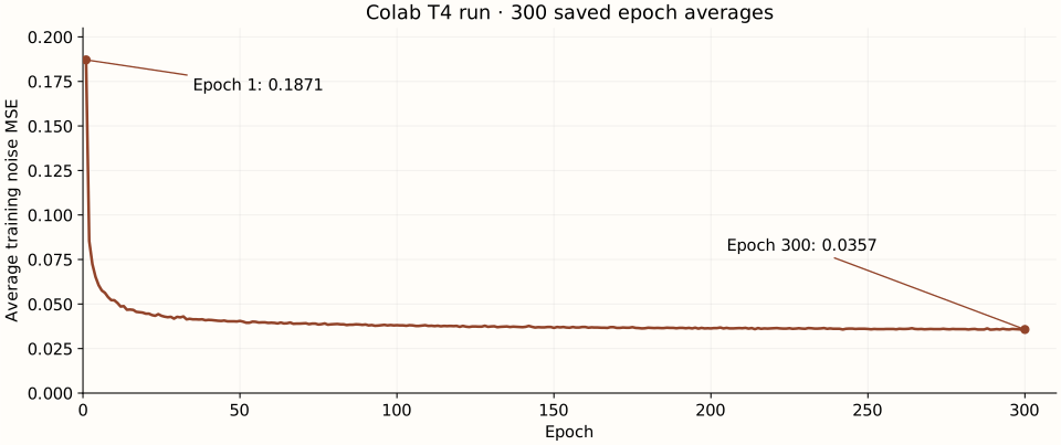
The latest run was trained on a Google Colab T4 GPU. The recorded notebook includes all 300 epoch logs, a successful checkpoint reload, and both generated-digit grids. The figures below are the saved outputs of that run; the loss curve is plotted from its recorded numbers.
9.1 Results from the completed T4 run
| Recorded setting | Value |
|---|---|
| GPU / device | Colab T4 / cuda |
| Learning rate / batch size | 1e-4 / 128 |
| Training epochs / batches per epoch | 300 / 469 |
| Diffusion steps / noise schedule | 300 / linear β from 1e-4 to 0.02 |
| First / final epoch-average noise MSE | 0.1871 / 0.0357 |
The run’s initial untrained-batch MSE was about 1.0473. After the first full epoch, the logged average was 0.1871; it reached 0.0521 at epoch 10, 0.0405 at epoch 50, 0.0381 at epoch 100, and 0.0357 at epoch 300. These measurements cover different points in training: an initial batch loss is not the same statistic as an epoch average.
For the first sampling cell, digits = list(range(10)) requests one image per class. The model starts from ten independent Gaussian noise tensors and runs the reverse chain while keeping each label fixed.

digits = list(range(10)), displayed with nrow=10. Read the requested classes from 0 to 9, left to right. These are the Colab results, not newly sampled images from a local checkpoint.For the second cell, digits = [7] * 16 holds the class constant while the random draws vary. The grid shows predominantly recognizable sevens with different slants, stroke widths, and top bars. Some samples are thicker or more distorted than others.
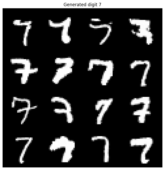
nrow=4. Variation comes from the sampled noise while the requested digit remains fixed.These outputs support a qualitative result: after this training run, the network can generate recognizable digit shapes and vary the handwriting within a requested class. They do not by themselves measure class accuracy or distribution coverage. The notebook records no FID, classifier accuracy, sampling seed, library versions, or total runtime, so no such values are attributed to these grids. The notebook hash, source cells, configuration, and image hashes are documented in the saved-run provenance file.
The recorded T4 notebook retains its original code, logs, and images. To train your own model, use the self-contained training edition: it adds epoch checkpoints, resume support, a loss plot, and diagnostics of noisy inputs, predicted noise, and implied clean images. Those diagnostics help connect the learned noise estimate to the generation results above.
9.2 Look at loss by noise level
Uniform timestep sampling mixes very different prediction problems into one scalar. At high noise levels, the input is dominated by noise, so copying a scaled version of the input can already be a useful noise predictor. At low noise levels, separating a tiny noise perturbation from fine digit structure is a different task. Neither a low overall MSE nor a monotonic-looking training curve is a complete generative-quality evaluation.
Use a fixed image batch and evaluate at t = [0, 30, 100, 200, 299]. Compare the predicted noise to the stored noise, then compute the implied x0 estimate. Include a zero-noise-predictor baseline and the exact-noise reconstruction. The exact-noise case should recover the image numerically; it validates the formula, not the trained network.
9.3 Questions that make a useful next experiment
| Observation | What to check next |
|---|---|
| Loss is NaN or shapes fail | Check finite schedule values, timestep bounds, broadcasting, devices, and that the output matches the noise tensor. |
| Loss is near 1 before training | Compare against the explicit zero-prediction baseline; this can be normal initialization behavior. |
| Training loss falls but generation looks poor | Inspect several seeds, per-timestep losses, the terminal α-bar, and whether the sampling schedule matches training. |
| Digits look plausible but ignore the requested class | With the same initial and intermediate random draws, change only the label. Inspect the learned conditioning path. |
| All sevens look alike | Try independent seeds and inspect a larger grid before drawing conclusions about diversity. |
| Resume starts again at epoch zero | Check the resume flag and checkpoint path; restore optimizer state as well as model weights. |
| CUDA assertion or CPU/CUDA mismatch | Rerun setup after selecting a GPU; keep the schedule, model, indices, and images on the same device. |
For a label comparison, reset the seed immediately before each complete sampling call so that both the initial noise and the later noise draws match. For a broader evaluation, add a held-out MNIST loader and report its timestep losses separately. A digit classifier can provide an additional label-consistency measurement, but this notebook does not include or claim that evaluation.
The lesson I wanted from this project is concrete: training learns a conditional noise estimate from synthetic supervised pairs; generation repeatedly uses that estimate inside a specified stochastic transition. Inspecting the data construction, loss target, and reverse coefficients is what turns “learn to denoise” into an algorithm you can debug.
10. Where each step comes from
Cell numbers below are one-based positions in the recorded 37-cell T4 notebook, including Markdown cells. The separate self-contained training edition adds explanations and inlines helpers, so its positions differ; use its numbered section headings to navigate.
| This post | Original cells | Original helper or action |
|---|---|---|
| Setup, configuration, data | 3–8 | Config, MNIST, show_images |
| Forward process | 9–12 | make_noise_schedule, extract, add_noise, visualizations |
| Time and label conditioning | 13–17 | sinusoidal_time_embedding, ConditionEmbedding |
| Residual blocks and U-Net | 18–27 | ResBlock, Downsample, Upsample, ConditionalUNet |
| Initial loss and backward check | 28–31 | F.mse_loss, diffusion_loss, AdamW |
| Training and checkpoint | 32–34 | train, torch.save, torch.load |
| Conditional generation | 35–37 | p_sample, sample_digits, sample grids |
The model architecture, linear schedule, noise target, original hyperparameters, and β-variance reverse sampler are preserved. Portability changes remove the private Drive dependency and hardcoded CUDA; presentation changes clarify indexing and display scaling. The training cell additionally provides epoch checkpoints, resume support, explicit AdamW defaults, and an image-weighted loss history. These conveniences belong to the self-contained edition. The reported T4 loss values and sample images come from the recorded notebook’s original training and sampling cells.