DIMES: A Differentiable Meta Solver for Combinatorial Optimization Problems

Zhen Tong Dec-20-2023

Introduction

Here is the corrected version:

This paper is written by Ruizhong Qiu from UIUC, and Zhiqing Sun∗, Yiming Yang from CMU Language Technologies Institute. The paper has been accepted by NeurIPS 2022.

This research focuses on the scalable problem in Graph Combinatorial Problems. Because Deep RL suffers from the costly decoding of COP solutions, the model encounters the sparse reward problem when dealing with large graphs. You can understand this by considering the construction of the graph or improving the graph to the final state as a very long trajectory because the graph is very large, and it only receives the reward at the end of the graph. Therefore, the reward is very sparse with respect to the long trajectory.

The researchers introduced a compact continuous space to parameterize the underlying distribution of candidate solutions, allowing massively parallel on-policy sampling without the costly decoding process. This effectively reduces the variance of the gradients by the REINFORCE algorithm. They also use meta-learning as an initialization of the model parameters.

DIMES can be generalized to problems, including locally decomposable combinatorial optimization problems, such as the Maximal Independent Set (MIS) problem for synthetic graphs and graphs reduced from satisfiability (SAT) problems.

Details

The novelty of DIMES compared to other construction heuristics learners is:

• Unlike previous methods which generate the solutions via a constructive Markov decision process (MDP) with rather costly decoding steps (adding one un-visited node per step to a partial solution), we introduce a compact continuous space to parameterize the underlying distribution of discrete candidate solutions and to allow efficient sampling from that distribution without costly neural network-involved decoding.

• Use meta-learning to train.

DIMES uses improving heuristics and unsupervised reinforcement learning.

Now we define the problem formally:

$\mathcal{F}_s$ is the set of all the solutions, $f$ is one solution, $s$ stands for an instance, $c_s()$ is the function for the solution $f_s$ cost. The solution space of COP is discrete, for example, the path of TSP, or the combination of MIS. However in the paper they parameterize the solution space with a continuous and differentiable vector $\theta\in\mathbb{R}^{|\mathcal{V}|_s}$, where $\mathcal{V}_s$ denotes the variables in the problem instances $s$, for example, edges in TSP and nodes in MIS, and estimates the probability of each feasible solution $f$ as:

where $p_\theta$ is an energy function over the discrete feasible solution space, $f$ is a $|\mathcal{V}_s|$-dimensional vector with element $f_i\in\{0, 1\}$indicating whether the $i^{th}$ variable is included in feasible solution $f$, and the higher value of $\theta_i$ means a higher probability for the $i^{th}$ variable produced by $p_\theta(f|s)$

Now the target function is the expectation over the continuous solution distribution for $f\sim p_s$

According to the REINFORCE-based update rule:

Nevertheless, a common practice to sample from the energy pθ functions
requires
MCMC(energy-based learning), which is not efficient enough. Hence we propose to design an auxiliary distribution qθ over the feasible solutions Fs, such that the following conditions hold: 1) sampling from $q_\theta$ is efficient, and 2) $q_θ$ and $p_θ$ should converge to the same optimal $θ^*$. Then, we can replace $p_θ$ with $q_θ$ in our objective function. $b(s)$ is the baseline.

Auxiliary Distribution For TSP

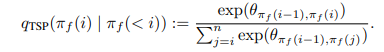
Only having a vector for the solution is not enough to describe the TSP solution. we need to add another distribution to describe the path. Because the TSP path is a ring, that can start from any point. Therefore

Given the start node $\pi_f(0)$, we factorize the probability via chain rule in the visiting order:

Auxiliary Distribution For MIS

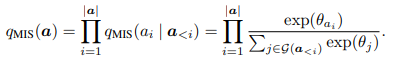
In the MIS problem, the solution is a set, but our sample is a vector, therefore we need to use a distribution to describe it.

$a$ is an ordering of the independent nodes in solution $f$, and $\{a\}_f$ is the set of all possible orderings of the nodes in $f$.

Meta-Learning

They train the GNN using the Meta-Learning conception. The idea is simple, select some graph instances and view them as tasks, and sample solutions for the graphs, after collecting many samples with gradients update the parameter for GNN

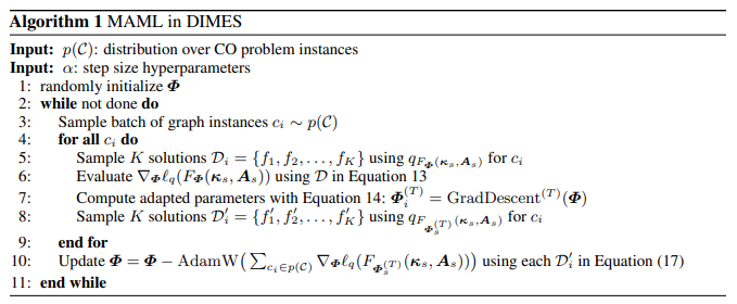
$\Phi$ is the parameter for the GNN, $K_s$is the input features for a graph instance $s$ in the collection $C$, $A_s$ si the adjacent matrix of the graph,

The meta-learning updates is:

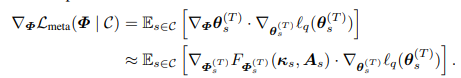
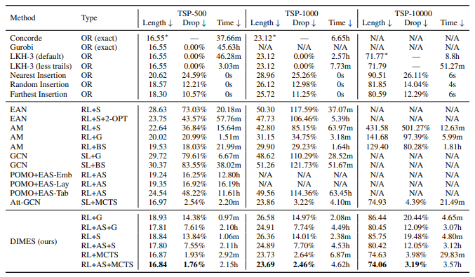
Performance